Researchers:
Fang Yih Chan
Faculty Advisor:
Dan Pirjol
Abstract:
The paper proposes the use of an Artificial Neural Network (ANN) to implement the calibration of the stochastic volatility model: SABR model to Swaption volatility surfaces or market quotes. The calibration process has two main steps that involves training the ANN and optimizing it. The ANN is trained offline using synthetic data of asset price generated by the Finite Difference Method and Dekker's root-finding method. The optimization is done to determine the optimal model parameters. This is done using the Inverse Map approach which utilize an inverse ANN and numerical calculation involving gradients of forward-pass ANN with respect to inputs. The proposed method is shown to efficiently and accurately calibrate high-dimensional stochastic volatility models like SABR.
Experiment:
Finite Difference Method:
The first step to obtain the implied volatility (IV) surface (data) is to compute the asset or option prices. The Black Scholes partial differential equation (PDE) derived through Feynman-Kac or Ito's Lemma enables the valuation of European options with underlying GBM stock via a closed-form solution. Similarly, the SABR model allows the valuation of a European option with underlying GBM volatility and the forward rate modeled as a Wiener process. The PDE for the SABR model is similar to the Black Scholes PDE, but with a two-dimensional structure and non-constant stochastic volatility. However, the SABR PDE cannot give a closed-form option value, so numerical methods such as Finite Difference Method (FDM) must be used. To reduce errors, a logarithm transformation is done by converting the PDE into a form with smaller coefficients. FDM has finite number of grids and requires artificial boundary conditions. Two types of boundary conditions are considered: Dirichlet and Neumann-boundary conditions, where the former assumes value is known or the later assumes derivative of function is known at the boundary.
Data:
To compute SABR option prices, actual market data is reviewed, which includes swaption data with different maturities, tenors, and strikes. Fixed levels of parameter values are used, and ten strike values with uniform spacing and two specific forward rates are chosen to generate all combinations of 14,400 data values. The maturities selected span from reasonably short term to long term that allow fitting of most available market data while maintaining a reasonable amount of computation time for data collection. FDM is used to compute option prices, which are then converted into implied volatilities using root-finding method on Black's equation. Specifically, Dekker's method is employed to avoid non-convergence or stalling when Secant or Bisection method alone is applied.
Calibration:
The purpose of using artificial neural network (ANN) in calibration to market data is to reduce the computational burden of pricing assets and allow the network to quickly approximate or predict prices online after training. The backward-pass step involves finding parameters that close the gap with market data using classical explicit minimization or optimization techniques such as LM or BFGS algorithm, DE technique or utilizing gradient information from the trained ANN to compute the search direction and solution. Alternatively, Inverse map approach is used, where an inverse ANN is established to solve the inverse problem of inputting market volatilities data to find the corresponding input parameters
ANN Construct:
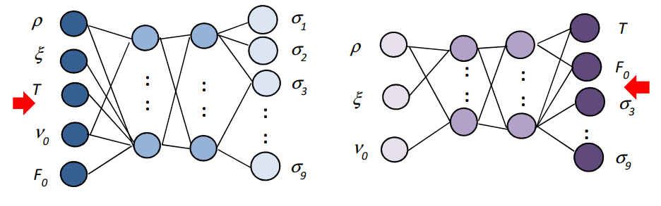
The forward ANN has two hidden layers with 160 nodes each, and the hyperparameters were determined via random search. The Adam optimizer with mean squared error (MSE) loss function was used for training with a learning rate of 0.001. The ReLU activation function was selected, and a dropout rate of 1/5 was applied to the first layer to reduce overfitting. The forward ANN takes five inputs, three of which are SABR model parameters (e, Vo, P), and two observable variables, maturity (T) and forward swap rate (Fo). The ANN has 9 outputs, corresponding to 9 fixed relative strike values with respect to the forward rate. The inverse ANN takes the output volatilities as inputs and still uses T and Fo as inputs. The original 3 input parameters are converted to inverse ANN outputs. The data sets were split randomly into training (80%) and testing (20%) sets.
Results:
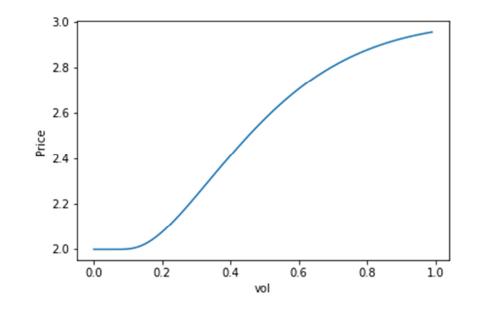
The implied volatilities derived from option prices that are computed using FDM are checked against Hagan’s approximation values. It is clear from the results that larger parameters tend to have higher RMSE, which is expected due to the higher nonlinearity introduced in the finite difference method. On the other hand, smaller parameters have a zig-zag curve, which is attributed to the difficulty in root-finding as Black's equation curve flattens at small volatilities.
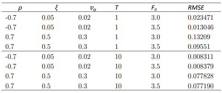
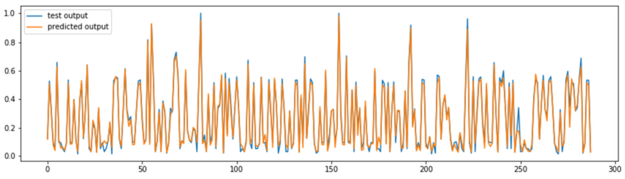
Longer maturity has a smaller RMSE compared to shorter maturity, which indicates better performance in terms of accuracy. Overall, the implied volatilities obtained from FDM have reasonably good values and can be used for training the ANN. The paper evaluated the performance of the trained artificial neural network (ANN) using Mean Squared Error (MSE) loss function, which measures the difference between predicted and actual values. The ANN was trained for 250 epochs, and the hyperparameters were chosen through K-fold cross-validation to minimize the MSE. The results showed that the ANN performed well, with MSE reduced to small values during training.
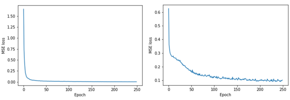
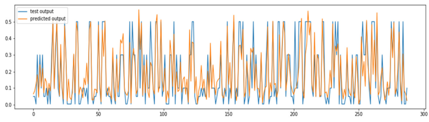
The forward ANN has a high explained variance of 99% for two out of the nine implied volatility outputs. Conversely, the inverse ANN has reasonable and acceptable explained variance of 66% and 77% for two of the outputs, ρ and ξ respectively, and a good explained variance of 99% for ν. However, the inverse ANN has less than ideal explained variance due to the possibility of multiple-to-one mapping between original input-output pairs, leading to the production of the average value of original ANN inputs. This is a limitation of the inverse ANN solver approach, which is greatly influenced by the combination of inputs and output values.
Calibration of SABR model parameters was done using daily swaption market data (implied volatilities) extracted from Bloomberg VCUB. The calibrated parameters were fed into the forward ANN to generate predicted implied volatilities to compare with the market quotes and the performance of calibration was evaluated using RMSE. This RSMEann was found to be 21.7%. If the calibrated parameters were used in Hagan’s approximation and the implied volatility values are compared with market quotes, the RMSE was found to be 18.7% and quite close to RSMEann.
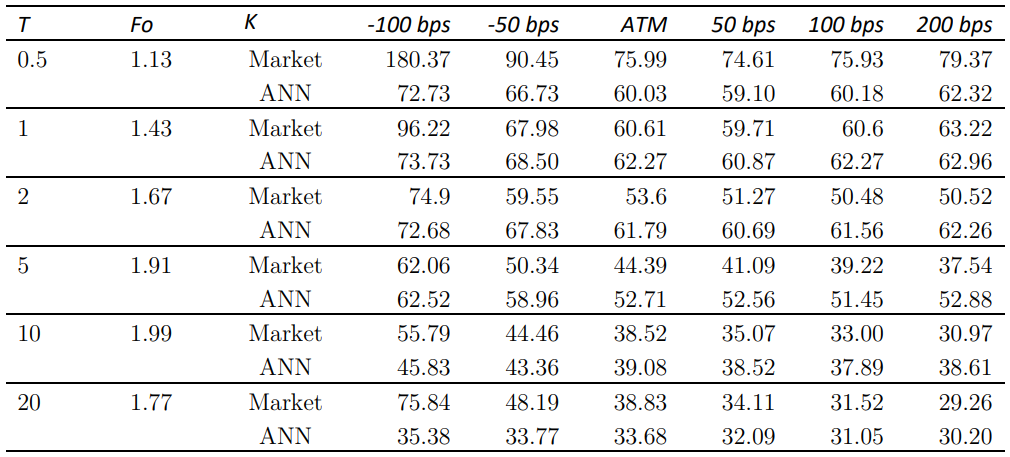
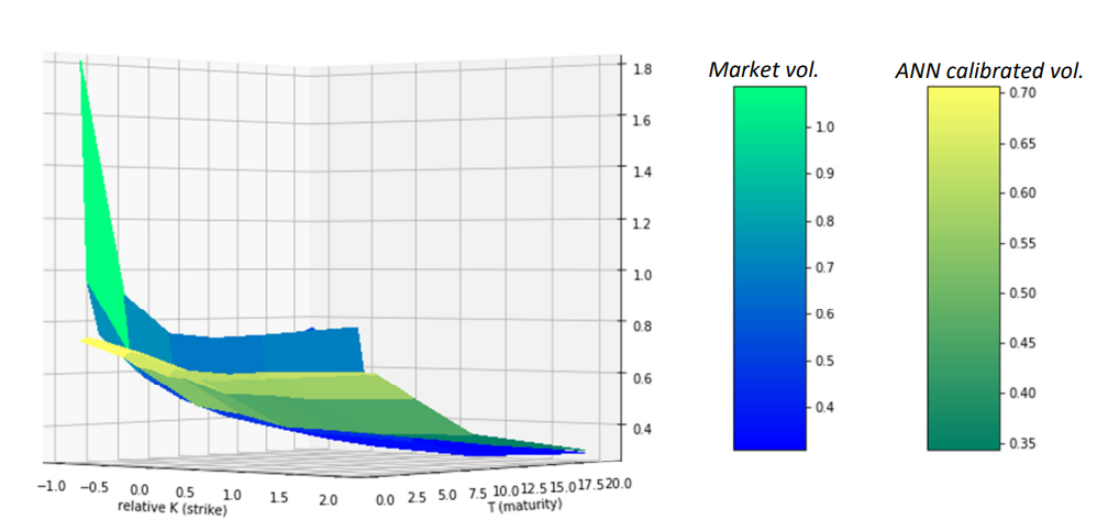
The RMSE for Hagan's approximation and ANN are 14.0% and 21.2% respectively, which are not too far off from each other. The calibration of SABR model parameters was extended to market data of other tenors (4Y, 6Y, 8Y, and 10Y) and the majority of calibrations showed good quality with RMSE around 10-15%. The paper also shows two-dimensional and three-dimensional (surface) plots of ANN predicted implied volatilities calibrated to fit with market quotes based on 2Y tenor data.
Conclusion:
This paper proposes using ANN to calibrate SABR stochastic volatility model to market volatility surface, providing a faster approach compared to traditional methods. The ANN utilizes two hidden layers with 160 nodes and ReLU activation function, and is trained using forward-pass stage, while the calibration process uses an inverse ANN with k-fold cross validation. The study shows promising results in calibrating to Swaption market implied volatilities with RMSE of 10-20%, using FDM implied volatilities consistent with Hagan's approximation. The study opens up avenues for future work, such as applying calibration to Futures Options market data or exploring different synthetic data generation methods.