Researchers:
Mathias Bantle
Faculty Advisor:
Dr Khaldoun Khashanah
Abstract:
Jumps in asset prices are not a new phenomenon, yet their incorporation into pricing models, trading strategies, and risk measures still leaves much to be desired. To facilitate the consideration of jumps in future research we conduct a comparison of several well-established as well as newly-developed jump identification techniques by examining their compatibility with a multivariate Hawkes process. Doing so, we identify two methodologies by Lee and Mykland and Khashanah, Chen, and Hawkes as being especially potent in empirically detecting jumps. The procedures provide us with a great amount of detail concerning the jump dynamics of our dataset of four equities and help us to describe the relationships between them. We discuss these findings along with an outline of the advantages and shortcomings of each method and provide guidance on how to conduct future research with respect to jump identification.
Introduction:
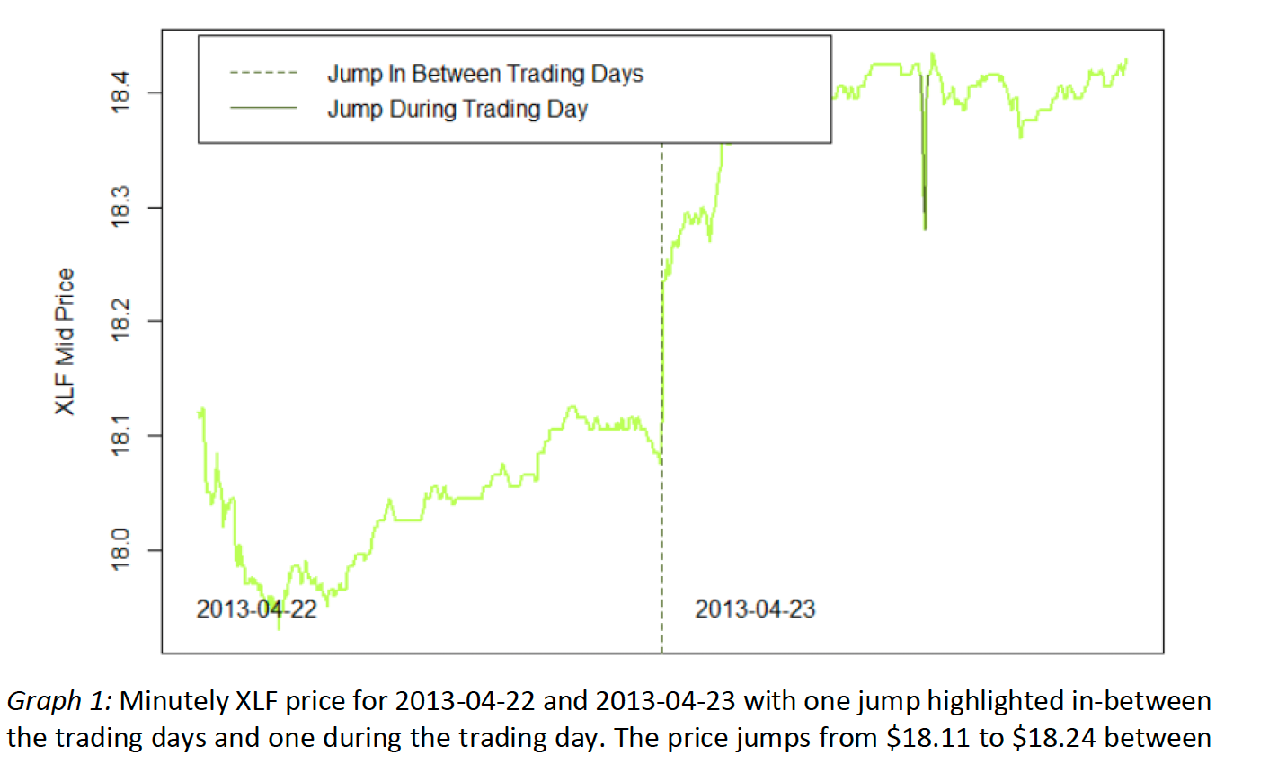
This passage discusses the concept of jumps in asset prices, specifically in financial markets, and introduces the objective of comparing four jump detection techniques. Jumps are defined as discontinuities in price processes, often observed between trading days. The paper aims to provide a rationale for jump detection techniques used in research by comparing established methods from Barndorrf-Nielsen and Shepherd, Huang and Tauchen, and Lee and Mykland, along with a newer technique from Khashanah, Chen, and Hawkes. The evaluation involves applying these techniques to a multivariate Hawkes process, measuring their detection accuracy through log-likelihoods and simulation statistics. The g-Hawkes process is emphasized as a tool to model jumps, with the paper organizing subsequent sections to review literature, introduce the dataset and techniques, present results, and conclude with implications for the study of financial jumps.
Literature on Financial Jumps and Hawkes Processes:
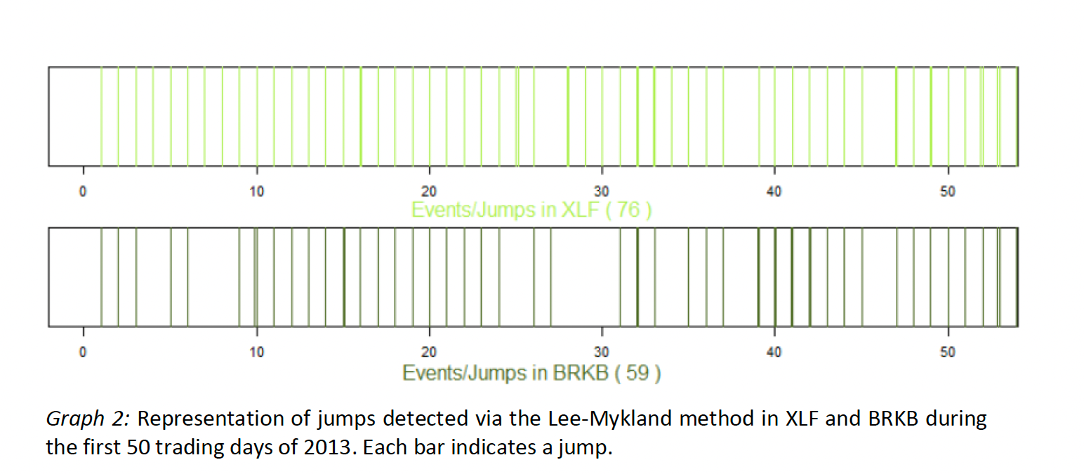
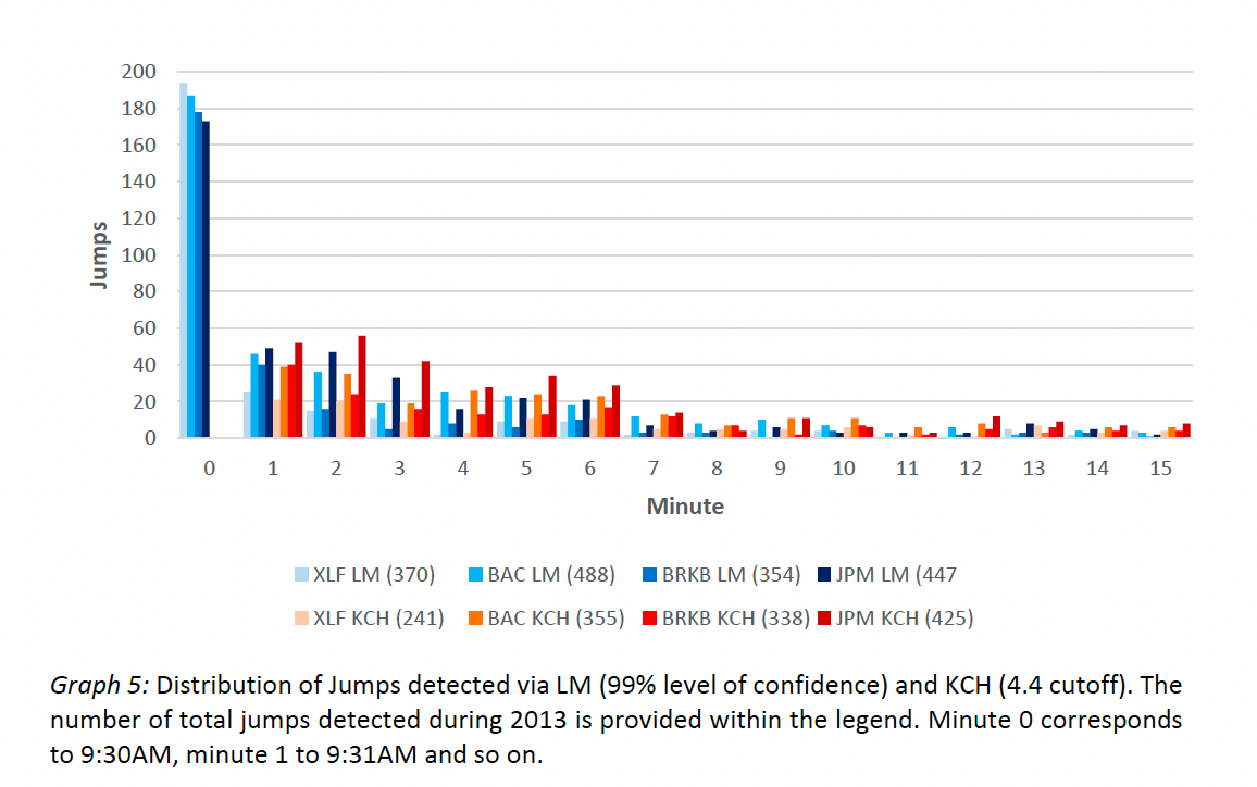
Hawkes processes, introduced by Alan G. Hawkes, are self- and mutually-exciting point processes, where the occurrence of an event increases the probability of subsequent events, resulting in clusters. The Lee-Mykland method is used to detect jumps in XLF and BRKB during the first 50 trading days of 2013. Hawkes processes find application in various disciplines, such as earthquake occurrence, urban crime development, and predicting tweet reshares.
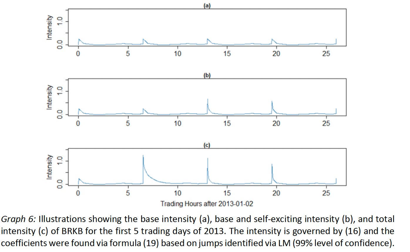
After the 2007-2009 Great Recession, there has been increased interest in Hawkes processes, particularly in quantitative finance. Khashahah, Chen, and Hawkes (2018) developed a dynamic Hawkes process that adapts its intensity to different trading day periods, capturing the observed U-shape in market activity. Their process models jumps in asset prices, and they discuss empirical jump detection using a flexible measure of daily realized variation.
Jump detection methods also include the KCH method and approaches based on bipower variation (BV), such as Barndorff-Nielsen and Shepherd (BNS), Andersen, Bollerslev, and Diebold (ABD), and Huang and Tauchen (HT). BV estimates the continuous component of realized variation, and differences between RV and BV help identify discontinuous (jump) contributions, with HT enhancing robustness to market microstructure noise.
Data and Methodology:
Dataset:
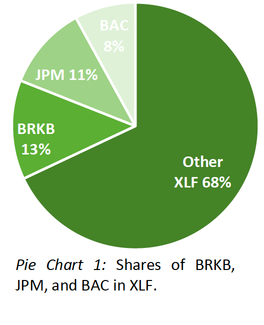
In times during which physical proximity to major exchanges, speed of broadband internet connections, and computing power can make a difference in succeeding or failing in security trading, working with weekly, daily, or hourly data may be outdated. Really, even the minutely (higher-frequency) observations used in our analysis are too coarse to be useful in algorithmic and high-frequency trading; yet, the findings based on our higher-frequency dataset may very well be generalized and then applied there. This dataset contains minutely observations of the highest bid, lowest ask, last, open, and close prices as well as volume and number of trades for the Financial Sector SPDR Fund (XLF) as well as its three largest constituents Berkshire Hathaway (BRKB), JP Morgan Chase (JPM), and Bank of America (BAC) that combined make up more than 30% of the index.
- RIC: Thompson Reuters Instrument code containing information on the equity in question and from which exchange its observations has been taken (in our case
- NASDAQ
- Datetime: Date and time of observation
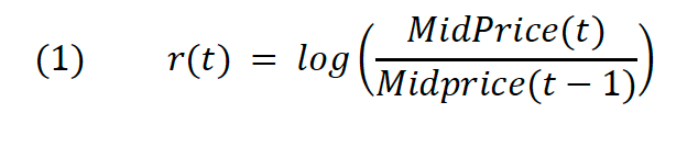
- Highest Bid & Lowest Ask: Used to calculate minutely mid prices and (log) returns
Jump detection:
Below outlines the implementation of the four jump identification methodologies used in this analysis and briefly discuss their characteristics. Note that the formulas in sections 3.2.1 and 3.2.2 come from HT, who provide a great summary of BNS and ABD while introducing their own jump detection measure. All other formulas are taken directly from the respective literature and were adjusted to conform to the context of this analysis where applicable. Furthermore, it is important to mention that the terms event and jump as well as return and log return are used interchangeably for the remaining discussion.
Barndorff-Nielsen and Shepherd (BNS) Jump Detection
BNS as well as ABD, HT, and LM consider a log-price process of the form
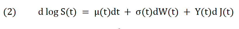
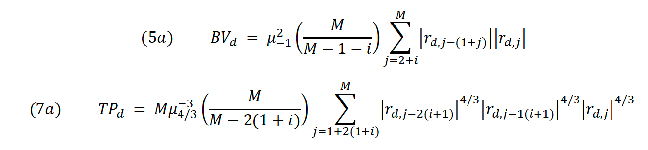
where μ(t) and σ(t) are the drift and diffusion terms and W(t) is a standard Brownian motion. Y(t) is the size of a jump, which is zero unless the jump counting (Poisson) process J(t) indicates the occurrence of an event. Assuming that J(t) and W(t) are independent of each other, BNS demonstrate how the variation in the price process (2) can be broken down into the sum of a continuous and discontinuous (jump) component where the discontinuous component can be measured by bipower variation. Total variation is represented by realized variation, which is the sum of all squared returns for a given period (usually a day d). BV is a measure of instantaneous variation.
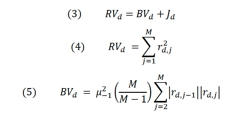
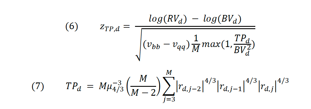
d is a given day, M the number of observations during that day, and 𝜇−12=𝜋2 . Notice that if we assume that equity returns are lognormally distributed and solve (3) for Jd the result is a difference between two sums of log returns, which is conveniently normally distributed. BNS (2005) take advantage of this and conduct a z-Test in order to identify significantly large values of Jd that are then considered to constitute a jump.
Huang and Tauchen (HT) Jump Detection
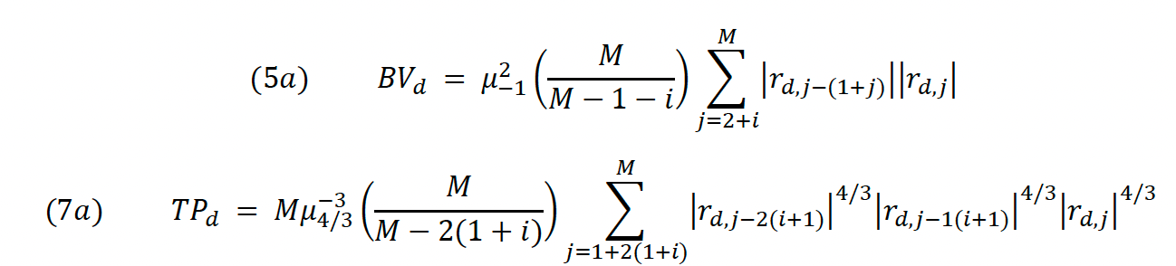
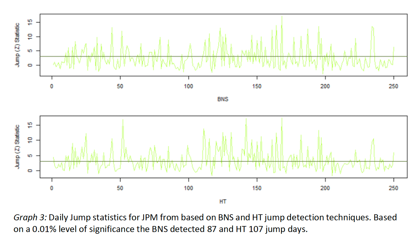
HT show in their paper how existing jump identification procedures (by BNS and ABD) are unprecise in identifying jumps as they tend to frequently overestimate or underestimate the jump component Jd. This happens due to market microstructure noise, which is variation in an asset’s price due to market dynamics rather than an actual movement of the equity in question. It is part of any empirical stock price time series that is not based on tick-by-tick data. The authors prove that using staggered instead of consecutive log returns in the calculation of (5) and (7) significantly reduces the effect of market microstructure noise on the jump statistic (6).
Lee, Mykland Method
In LM, the authors also use bipower variation in order to measure instantaneous volatility; however, instead of finding a single BV for each trading day, they find a rolling BV for each observation (in our case minute) in the dataset. Then they scale (divide) each log return by its associated BV and like this find what is referred to as the L-Statistic:
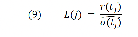
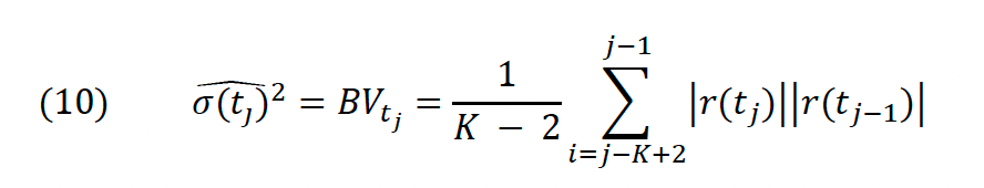
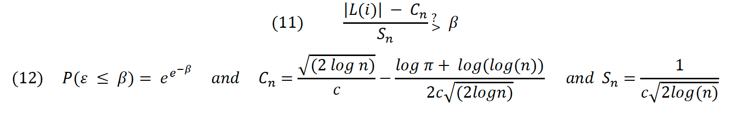
The formula for K assures that jumps preceding an observation at minute t do not impact the volatility measure significantly and so do not “cover up” a potential jump at t+1. Therefore, the L-statistic measures the relative size of the current return to the root of the sum of all previous K squared returns. To find a cutoff point at which that size is large enough to constitute a jump, the following L-Test (11) is conducted:
Khashanah, Chen, Hawkes Method
While LM measure instantaneous volatility via a rolling, localized, backwards-looking version of bipower variation, KCH use a realized volatility measure that is held constant during a given day. It is an estimator for realized variation (4) based on the sum of rolling medians from n consecutive observations on a given day:
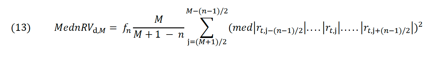
In (13), M is the number of observations per day while n may be dynamically chosen. Typical values for n are 5, 7, and 9 observations with fn of 1.6236, 1.74332, and 1.82184 respectively. In the analysis n = 9 is used, which is most suitable when working with higher-frequency data.
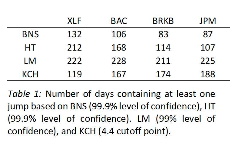
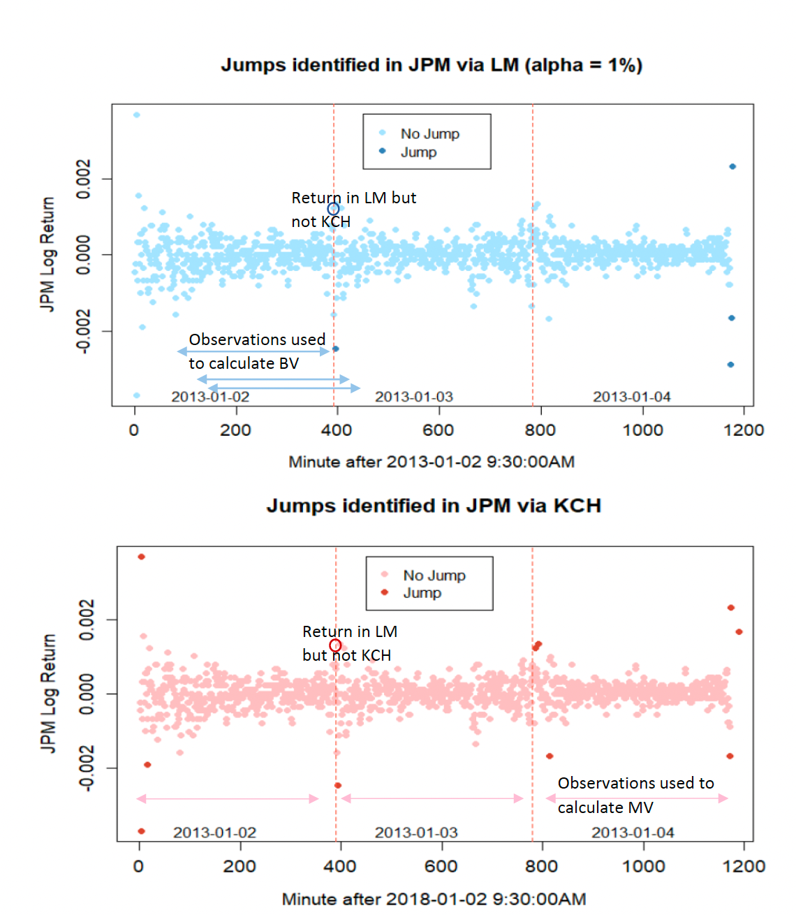
The BNS and HT jump discovery procedures are despite their importance in research pertaining to jump identification too simplistic for our analysis. Therefore, our comparison will focus on the LM and KCH methods, which can identify any given return as jump or no jump.
Model Calibration
Multivariate g-Hawkes Process
According to the literature, both the LM and KCH method are expected to robustly identify jumps, reduce the chance of large jumps overshadowing smaller, successive jumps, and should work especially well within Poisson-type jump processes. KCH even suggest that their MV measure also improves the Lee and Mykland (2008) method as if avoids masking effects (2018, 4). Whether this is true or not will be answered by calibrating the multivariate g-Hawkes process by Bowsher (2007) based on the jumps detected, assessing the resulting model fit based on log- likelihood, Box-Ljung tests, and simulation.
Maximum Likelihood Estimation (MLE)
The attentive reader realized that, in order to calibrate our g-Hawkes process based on our empirically identified jump times, we need to find estimates for a total of 4*24=96 parameters from each the LM and KCH jump times. This task is anything but trivial and extremely time consuming. Fortunately, Bowsher provided a log-likelihood function along with his process that facilities this estimation.
Model Fit
To assess the goodness of fit of the empirically identified jump times based on LM and KCH to Bowsher’s g-Hawkes process, log likelihood is examined and Box-Ljung tests as well as perform simulation. Jump-detection method is expected to yield the higher likelihood to have the better fit. Box-Ljung tests check whether there is autocorrelation in a time series. A positive test (autocorrelation) indicates that there is a significant lack of fit in the model.
Conclusion
The analysis aimed to identify a jump detection methodology for future research on jumps and jump processes. Among the considered techniques, the KCH and LM methods were recognized as the most flexible and dynamic. Both methods revealed a Hawkes process indicating that the intensity of Berkshire Hathaway is influenced by its own jumps and jumps in the XLF index, although the two processes differed in characteristics. The LM method exhibited greater precision in jump identification based on log-likelihood, while the KCH method demonstrated higher accuracy in a simulation. The recommendation is to extend the analysis before making definitive conclusions, suggesting exploration with a larger dataset, ultra-high-frequency data, in a higher-dimensional setting, and with different assets and events. The attached R code provides the necessary functionality for such extended analyses.