Researchers
Andrew Kaminsky
Ravi Patel
Bryce Streeper
Faculty Advisor
Prof. Khaldoun Khashanah
Abstract
The authors conducted a project on Robo-risk and Copula CoVaR of SPY, aiming to analyze the systemic risk of the S&P select sector ETFs and SPY. They utilized intraday data for 2010 and daily data from 2006 through 2022. VaR (Value at Risk) was calculated for each ETF using both empirical distribution and Gram-Charlier distribution methods. SPY was treated as a system of sector ETFs, and ΔCoVaR was calculated accordingly. Finally, the authors identified an approximating copula to the joint distribution of returns. The project was motivated by the growing importance of risk management in financial markets, aiming to offer valuable insights for investors and portfolio managers interested in SPY and sector ETFs.
Methodology
Data Collection
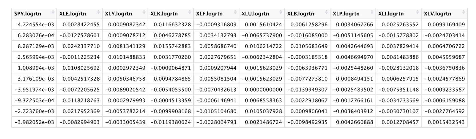
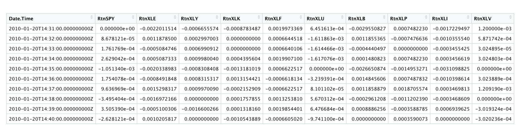
The initial phase of the project involved gathering data on the performance of SPY and various sector ETFs: SPY, XLE, XLY, XLK, XLF, XLU, XLB, XLP, XLI, and XLV ETFs. Data acquisition was conducted using Yahoo Finance for daily data and Bloomberg Terminal for intraday data. Intraday data with a one-minute frequency for the year 2010, the most detailed level available, was obtained from Bloomberg Terminal. The data underwent sanitization, including the creation of UTC and EST hour and minute columns, filtering values to encompass market hours (9:30 am to 4:00 pm), and computation of log and simple returns. Returns from each index were consolidated into a single CSV file for subsequent analysis.
Similarly, the daily dataset, covering daily return data from 2006 to 2022, was processed in a similar manner. Log and simple returns were computed for this dataset as well. Below is a snippet of the daily data and intraday data:
Value at Risk
Value at Risk (VaR) is a statistical metric assessing the potential financial risk within a portfolio or investment over a specific time frame. It estimates the maximum potential loss a portfolio might experience within a given period at a certain confidence level. In this project, VaR is computed for each ETF and SPY individually over a ten-day period using two distribution techniques: empirical distribution and Gram-Charlier distribution expansion. The aim is to compare these methods for their viability in CoVaR, ΔCoVaR, and Copula calculations.
The 95% VaR, 99% VaR, and Median Return (50% confidence level) are calculated for each index across different time intervals (e.g., 15 minutes, daily, weekly) to compare the effects of time periods and confidence intervals. The empirical distribution technique employs historical data to estimate return probability distribution, making it valuable when the underlying distribution is unknown or non-normal. The process involves ranking historical returns and selecting the nth percentile as VaR.
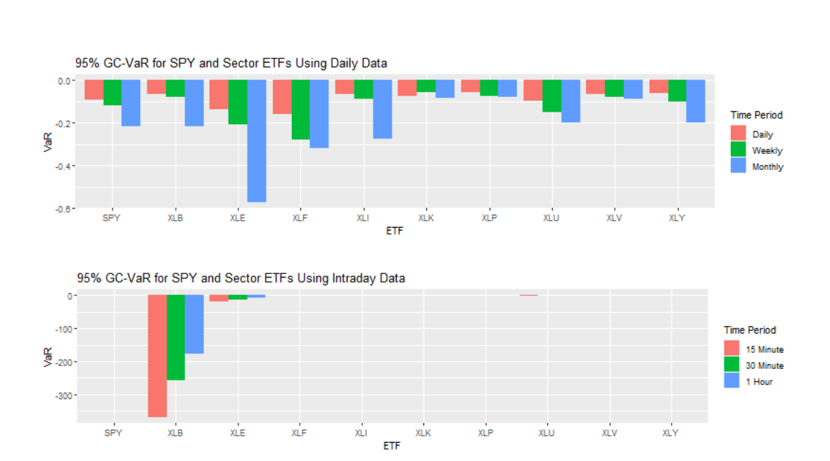
Visualizations below illustrate the 95% VaR for SPY and Sector ETFs using daily and intraday data to better understand the relationships between time intervals and confidence levels.
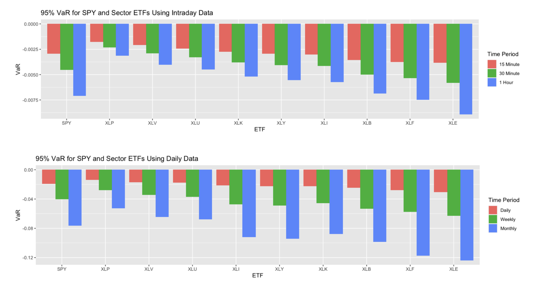
The empirical VaR values calculated are all negative but relatively low, while the median returns are positive. This suggests minimal risk and a high likelihood of short-term gains if one invests in each index. Additionally, there's a noticeable pattern: as the time period increases, so does the calculated VaR, indicating higher implied volatility and a greater risk potential over longer periods.
The second method, the Gram-Charlier distribution, estimates risk by utilizing characteristic functions to approximate return distributions. It's particularly useful for skewed and leptokurtic distributions. This method incorporates conditional mean, volatility, and a probability density function of Psi, integrating skewness and kurtosis. Unlike the empirical distribution that relies on historical data, the Gram-Charlier Distribution employs a mathematical formula to estimate VaR.
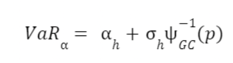
This function takes into account the mean and variance of a portfolio, as well as the inverse of Ѱ, the Gram-Charlier expansion, of probability p, which in terms of k is:

Where: Φ is the standard normal CDF, φ is the standard normal PDF, 𝑘 is the skewness of the 3 portfolio, and 𝑘 is the kurtosis of the portfolio. As well, the inverse of the GC was taken by the interval 4 -inf to z, where z is the confidence interval specified. By estimating the parameters of the GC-distribution for each ETF given the calculated mean, variance, skewness, and kurtosis values of each ETF, the inverse cumulative distribution of the estimated GC calculation at the 95% confidence level can be observed:
ΔCoVaR Analysis of SPY as System of Sectors
Calculations
CoVaR and ΔCoVaR are systemic risk measures used to quantify the systemic risk of a part of the system on the entire system. In our case the system is the entire stock market (the SPY ETF), and the parts of the system are the sector ETFs. CoVaR and ΔCoVaR are calculated using the historical VaR values covered earlier, using these two equations for CoVaR and ΔCoVaR respectively:
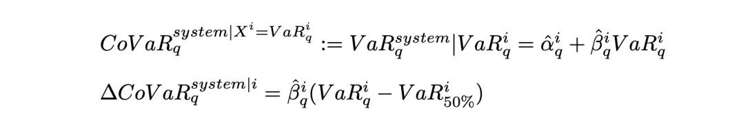
The α and β values in the equations are derived by regressing the log returns of each sector ETF onto the log returns of the system (SPY). CoVaR indicates how the system responds when a part of it hits its VaR threshold, typically focusing on the 95% VaR. For instance, the 95% CoVaR of SPY concerning XLE reflects the SPY's reaction if XLE drops to its 95% VaR value.
ΔCoVaR provides a more comprehensive view of systemic risk by considering the median value of the system. It is calculated as the difference between the 95% CoVaR of the system and the 50% CoVaR of the system. ΔCoVaR illustrates how the system reacts when one part hits its 95% VaR relative to its median value. This metric is particularly insightful for sector ETFs with median values above zero, as it indicates changes concerning the ETF's normal performance rather than when it has a return of 0%. The use of ΔCoVaR offers clearer insights into systemic risk, especially considering the varying median returns among sector ETFs. As a result, ΔCoVaR is considered the primary indicator of systemic risk in this context.
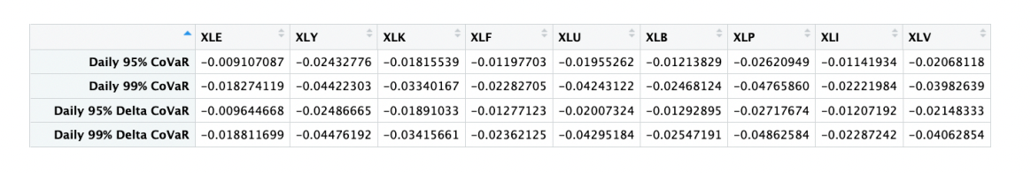
Above is a table of 95% and 99% daily CoVaR and ΔCoVaR values for the entire dataset from 2006 through 2022. To give a clearer idea of what CoVaR and ΔCoVaR are, if XLE hits its 95% VaR, the returns of the SPY are expected to be -0.91% (daily 95% CoVaR value), and the returns of SPY in comparison to when XLE is at its median value are expected to be -0.96%.
Analysis
The analysis of ΔCoVaR is segmented into four sections: the entire daily dataset spanning from 2006 to 2022, the daily dataset during recessions, the daily dataset during bull markets, and the intraday data comprising one-minute log returns for 2010. Examining the entire daily dataset provides insights into the differences among ETFs. It's crucial to consider each sector's riskiness, as sectors with higher VaR are likely to exert a more significant impact on the overall market compared to less risky sectors. Additionally, assessing market conditions, whether in normal operations or during a recession, is essential.
The graph below illustrates VaR against ΔCoVaR for each sector throughout the daily dataset. Data points for all dates are depicted in blue, while those during bull markets are in green, and values during recessions are in red. This color-coded representation aids in understanding the dynamics of systemic risk across different market conditions and sectors.
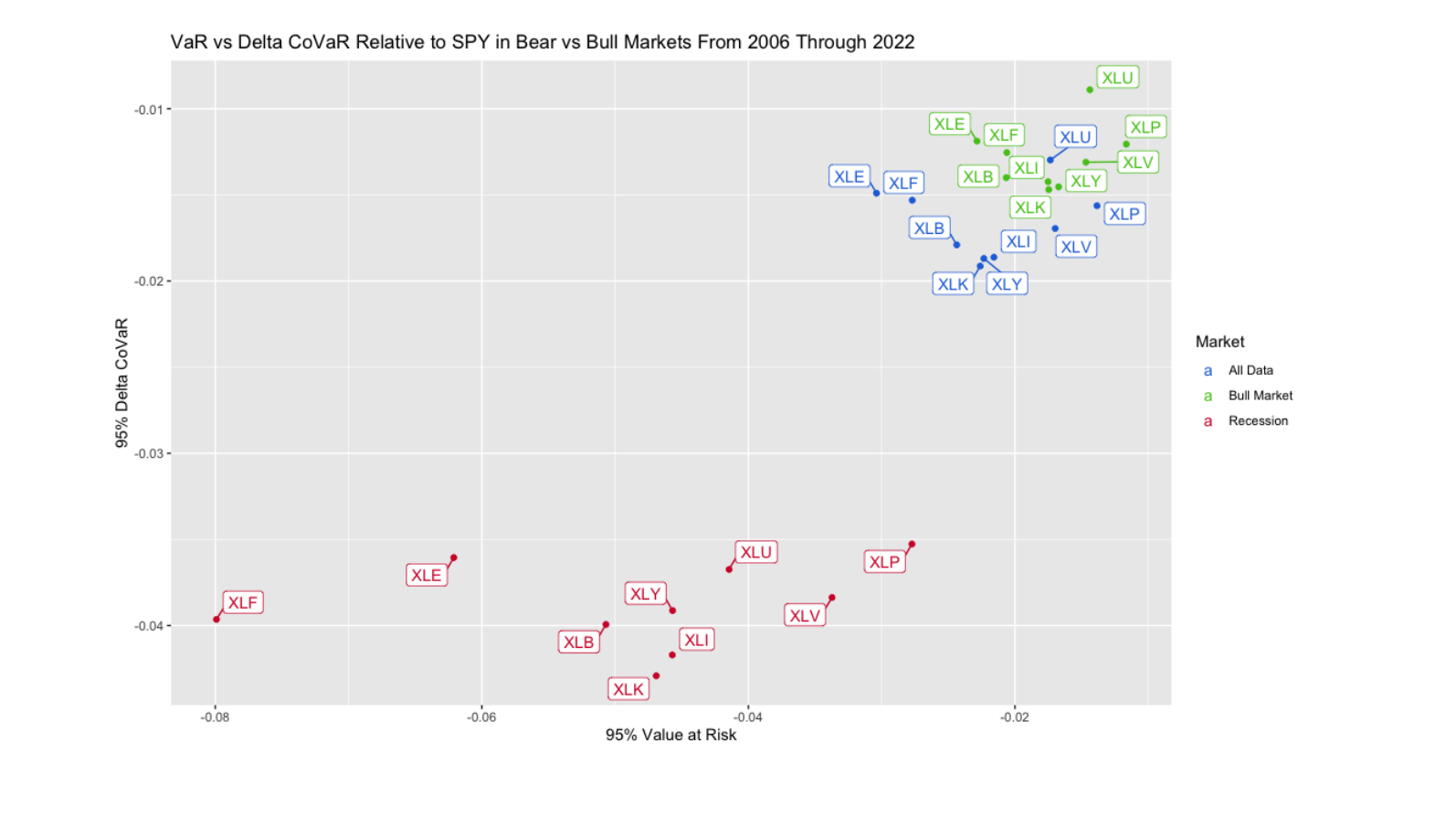
bull markets, indicating higher risk levels. The entire dataset values, depicted in blue, fall between the bull market and recession data points, aligning with expectations. Recessions make sectors and the market more susceptible to negative swings, increasing overall risk. To offer deeper insights into the systemic risk dynamics across different market regimes, analyzing the ratio between VaR and ΔCoVaR for each sector may prove more informative.
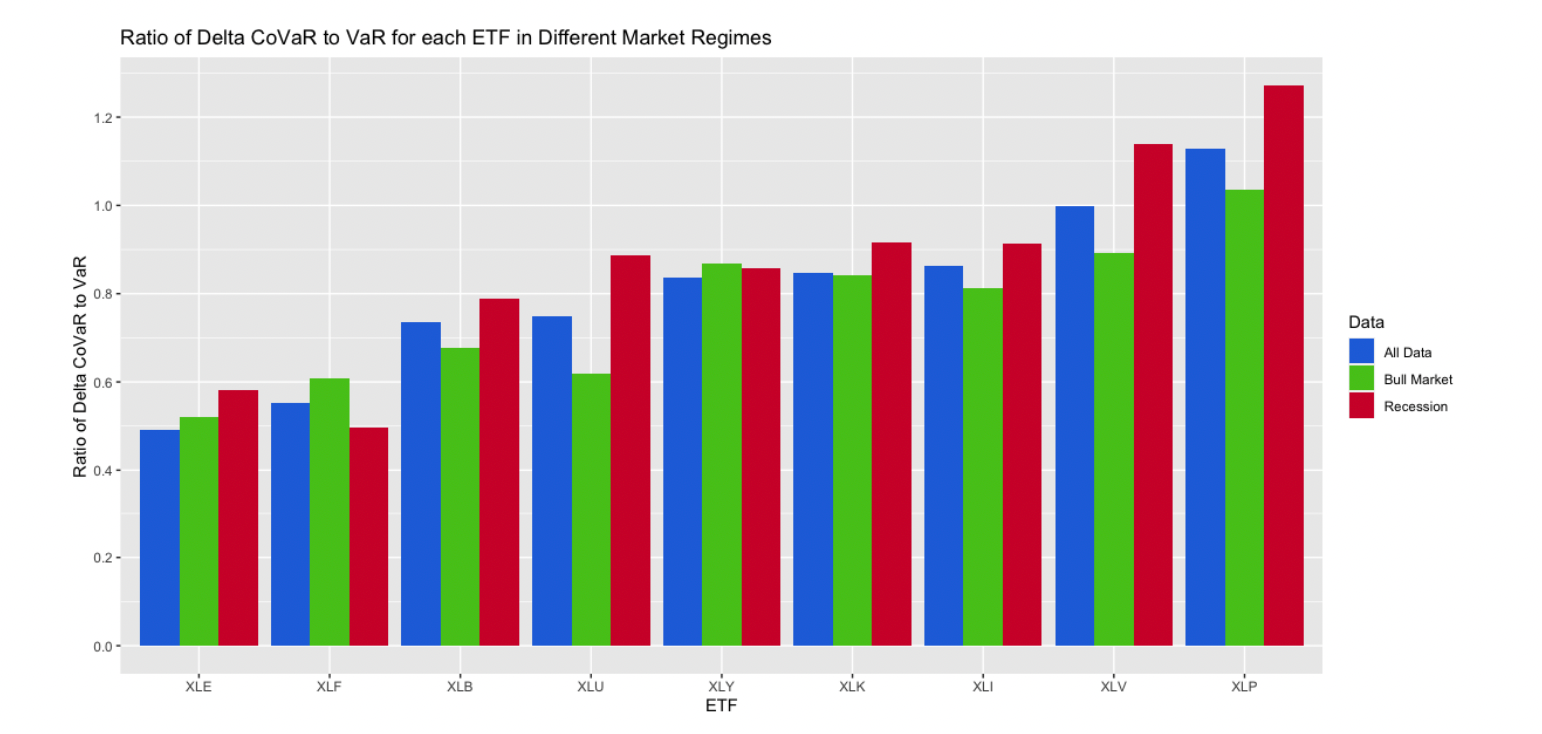
Analyzing the ratio of VaR to ΔCoVaR for each ETF across various market regimes provides insights into sectors' impact on the market. Sectors like technology, industrials, and consumer discretionary consistently exhibit high ΔCoVaR relative to VaR. Conversely, less risky sectors like consumer staples and healthcare display higher ratios of VaR to ΔCoVaR. Financials and energy, despite being the riskiest sectors, have the lowest ratio of VaR to ΔCoVaR and aren't among the highest for ΔCoVaR itself. Utilities and materials consistently rank lower in VaR, ΔCoVaR, and their ratio.
These results suggest that movements in less cyclical and less risky sectors like consumer staples and healthcare may signal broader market issues, while movements in energy and financials often remain localized. Further analysis should delve into the characteristics of the two recessions since 2006 and explore differences before and after these recessions. Understanding how recessions impact systemic risk dynamics and how markets evolve post-recession will offer valuable insights into market behavior and risk management strategies.
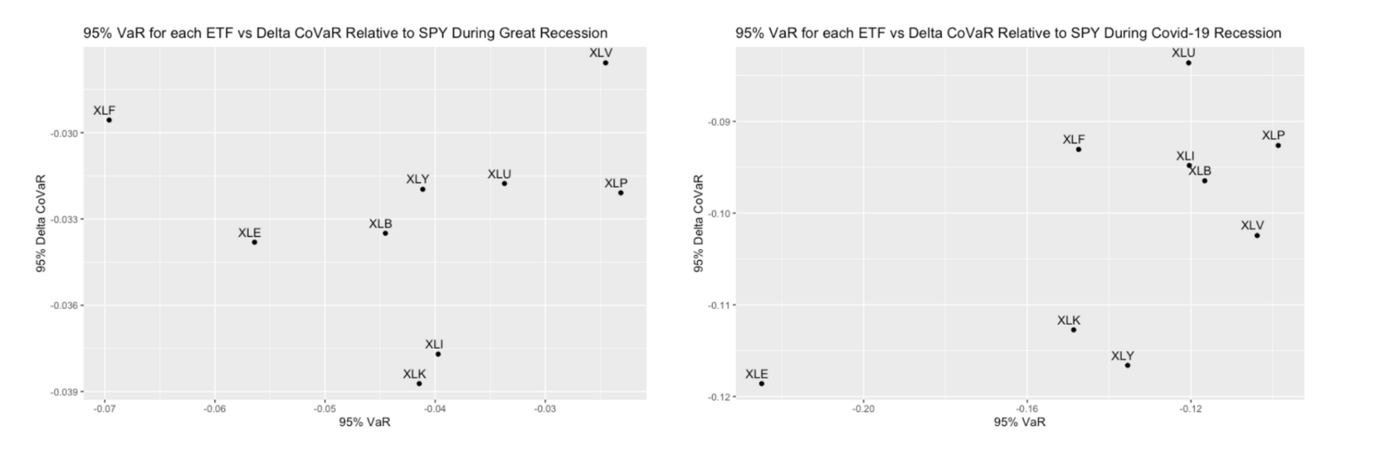
Examining each recession reveals distinct differences in the sectors most affected. Financials experienced the highest VaR during the Great Recession, while energy had the highest VaR during the COVID-19 recession. Interestingly, during the Great Recession, financials had the second-lowest ΔCoVaR, whereas during the COVID-19 recession, energy had both the highest VaR and ΔCoVaR. However, the ratio of VaR to ΔCoVaR for energy wasn't as remarkable, possibly due to the severity and duration of the impact.
Apart from these differences, few similarities exist between the two periods, except for consumer staples remaining relatively stable and technology consistently ranking high in ΔCoVaR. The dissimilarities likely stem from variations in causes and market impacts of each recession. Additionally, the axes for the COVID-19 recession are notably larger, reflecting its longer duration compared to the Great Recession. Next, analysis will focus on bull markets before, after, and between the two recessions in the time period.

Across all bull markets, consumer discretionary, industrials, and technology consistently exhibited the highest ΔCoVaR, while utilities and consumer staples ranked among the lowest. Despite having the highest VaR overall, energy tended to have lower ΔCoVaR. Before the Great Recession, financials had the highest ΔCoVaR, indicating the market's strong reaction to changes in this sector, but this decreased post-recession, possibly due to shifts in market dynamics and consumer sentiment.
Similarly, the materials sector experienced a moderate decrease in VaR and ΔCoVaR after the COVID-19 recession, mirroring the trend observed with financials after the Great Recession. Over time, both VaR and ΔCoVaR values increased, indicating a gradual rise in market risk. This increase may be attributed to changes in market sentiment and dynamics following the recessions, leading to more frequent and significant market swings.
Next, the analysis will focus on intraday ΔCoVaR to further explore systemic risk dynamics.
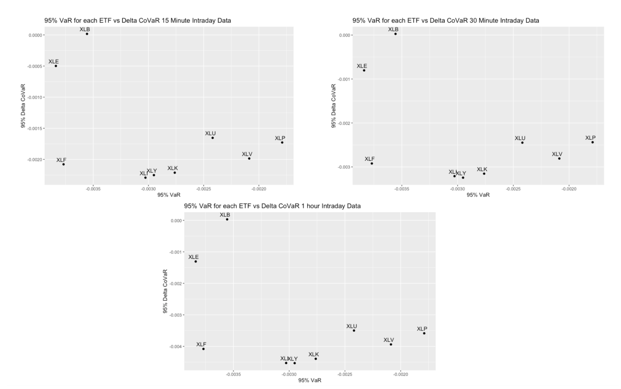
The intraday data analysis from 2010 reveals some notable differences compared to the daily data analysis between the two recessions. In intraday data, utilities exhibit a significantly higher ΔCoVaR, while materials display lower systemic risk and higher VaR. The remaining ETFs generally align with patterns observed in daily data.
Interestingly, most sectors show similar ΔCoVaR values in intraday data, except for energy and materials, which exhibit lower ΔCoVaR despite having higher VaR. This indicates that while energy and materials are riskier, they don't impact the SPY as significantly as other sectors. These observations shed light on the nuanced dynamics of systemic risk across different time frames and highlight variations in sectoral impact on the overall market.
Results
The ΔCoVaR analysis of the SPY and sector ETFs reveals several insights into systemic risk dynamics over the studied period. Consumer staples and healthcare consistently exhibit the highest ratio of VaR to ΔCoVaR, indicating that changes in these sectors often signify broader market issues. Conversely, financials and energy have the lowest ratio, suggesting that changes within these sectors are typically isolated issues rather than systemic concerns.
During each recession, distinct market dynamics translate into varied ΔCoVaR values for sectors. Financials were notably risky during the Great Recession, while energy stood out during the COVID-19 recession. However, financials didn't exhibit high ΔCoVaR during the Great Recession compared to other sectors.
Analysis before, after, and between the recessions reveals shifts in systemic risk dynamics, notably seen in financials post-Great Recession and materials post-COVID-19 recession. Moreover, over time, both individual sectors and systemic risk have increased, reflecting evolving market conditions and sentiment.