Researcher
Gordon Garisch, M.S. in Financial Analytics, Graduated in May 2020
Advisor:
Dr. Zachary Feinstein
Abstract
In this project we use as staring point a the measure of systemic risk as the set of allocations of additional capital to each entity in a financial network that leads to acceptable outcomes to the beneficiaries of that network. Utilizing a standard Eisenberg-Noe framework for this network, we propose several combinations of machine learning models and simulation procedures that can be used in the determination of efficient and acceptable capital allocations. We explore the accuracy and computational efficiency of logistic regression with various kernel specifications as well as basic neural networks in this regard. We further show the impact of utilizing Gibbs sampling in the simulation of capital allocations. Our methodology is applied to a dataset of European banks where we find that basic neural networks provide more accurate and computationally efficient allocations of capital than logistic regression under various kernel specifications.
Keywords: Systemic risk, Eisenberg-Noe clearing vector, Machine learning
Approach
Using 4 candidate models, as outlined in table 1, a dataset of 87 banks based on European bank stress tests, as derived by Feinstein et al. (2018), and the framework for a financial system proposed by Eisenberg and Noe (2001), we set out to solve for optimal capital allocation among 87 banks in a tiered capital system.
| Description | Specification |
|---|---|
| Logistic | $${\Pr(Y=1|K=k)=\frac{1}{1+e^{-\phi(\beta,\gamma,k)}} \\ \text{where: }\\\phi(\overline{\beta},\overline{\gamma},\overline{x})=\beta_0+\sum_{i=1}^{n}{\beta_i x_i}}$$ |
| Logistic Including Interaction Variables |
$${\Pr(Y=1|K=k)=\frac{1}{1+e^{-\phi(\beta,\gamma,k)}} \\ \text{where: }\\\phi(\overline{\beta},\overline{\gamma},\overline{x}) =\beta_0+\sum_{i=1}^{n}{\beta_i x_i}+\sum_{i=1}^{n}{\sum_{j=i+1}^{n}{\gamma_i x_i x_j}}}$$ |
| Logistic Interaction Variables Only |
$${\Pr(Y=1|K=k)=\frac{1}{1+e^{-\phi(\beta,\gamma,k)}} \\ \text{where: }\\\phi(\overline{\beta},\overline{\gamma},\overline{x}) =\beta_0+\sum_{i=1}^{n}{\sum_{j=i+1}^{n}{\gamma_i x_i x_j}}}$$ |
| Simple Neural Network |
Basic neural network with one hidden layer containing one node for each tier in the banking system |
Table 1: Candidate Model Summary
The number of tiers in the banking system determines the dimensionality of the optimization problem. In a two-tiered system, each of the 87 banks can only have two percentages of capital allocation, i.e. a capital allocation vector k = (k1, k2). In a three-tired system the allocation vector becomes k = (k1, k2, k3), etc.
To allow alignment to real world regulatory regimes, the allocation is based on the size of Assets Under Management (AUM) with similar sized banks grouped together. Each tier in the system is designed to contain similar amounts of AUM. Table 2 illustrates the tiering for a select number of capital allocation tiers, along with the total percentage of AUM for each group.
| Capital System Description | Capital Allocation Grouping |
|---|---|
| 2-Tiered | $$ (\underbrace{1,2,3,4,\cdots,9}_{\stackrel{k_1}{\text{48.1%}}},\underbrace{10,\cdots,87}_{\stackrel{k_2}{\text{51.9%}}})$$ |
| 3-Tiered | $$(\underbrace{1,2,\cdots,5}_{\stackrel{k_1}{\text{32.5%}}},\underbrace{6,\cdots,16}_{\stackrel{k_2}{\text{33.7%}}},\underbrace{17,\cdots,87}_{\stackrel{k_3}{\text{33.8%}}})$$ |
| 4-Tiered | $$(\underbrace{1,2,3}_{\stackrel{k_1}{\text{20.7%}}},\underbrace{4,\cdots,9}_{\stackrel{k_2}{\text{27.4%}}},\underbrace{10,\cdots,21}_{\stackrel{k_3}{\text{26.3%}}},\underbrace{22,\cdots,87}_{\stackrel{k_4}{\text{25.7%}}})$$ |
| ... | ... |
| 87-Tiered | $$(\underbrace{1}_{\stackrel{k_1}{\text{7.3%}}},\underbrace{2}_{\stackrel{k_2}{\text{6.9%}}},\cdots,\underbrace{86}_{\stackrel{k_{86}}{\text{0.003%}}},\underbrace{87}_{\stackrel{k_{87}}{\text{0.001%}}})$$ |
Table 2: Allocation Groupings and AUM Per Group Per Number of Tiers in Capital System
The problem of optimal capital allocation is defined by identifying a vector k based on the acceptance criteria A using the framework provided by Feinstein et al. (2017). To be more specific, the acceptance criteria is defined as:
A = {k ∈ Rn∣ES(r + p ⋅ k) ≤ 0.98 × Obligation to Society}
where ES is Expected Shortfall, and p and r are the proportional nominal liabilities, and external cashflows, respectively, as per Eisenberg and Noe (2001).
In this approach, the values of vector k are sampled from a Uniform distribution on the domain (0,1), as well as through Gibbs sampling. The purpose of multiple sampling techniques is to speed up convergence and to assess computational efficiency.
Main Results
Convergence
The outcomes are shown in figure 1. The results tend to show faster convergence when using Gibbs sampling and that the logistic regression model that includes interactions and the neural network have the lowest losses. The neural network models show the best performance overall.
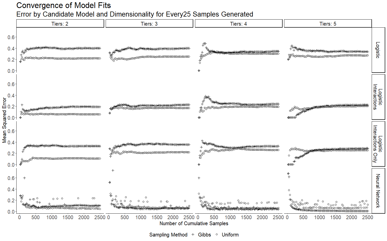
Additionally, the losses appear to increase slightly as dimensionality increases, but do not appear to scale exponentially, or even linearly. This suggests that the approach would be well suited to an increase in dimensions.
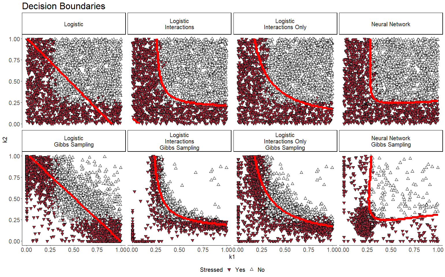
To supplement this information, we can also observe the shape of the decision boundaries produced by these models in 2 dimensions. This is shown in figure 2. These clearly show the enhanced sampling pattern produced through Gibbs sampling. It also highlights limitations of certain candidate models. Simple logistic regression is not able to account for non-linearity while the logistic regression with an expanded kernel that includes inter- actions variables introduces non-monotonicity (this is evident in row 1, column 2 of figure 2).
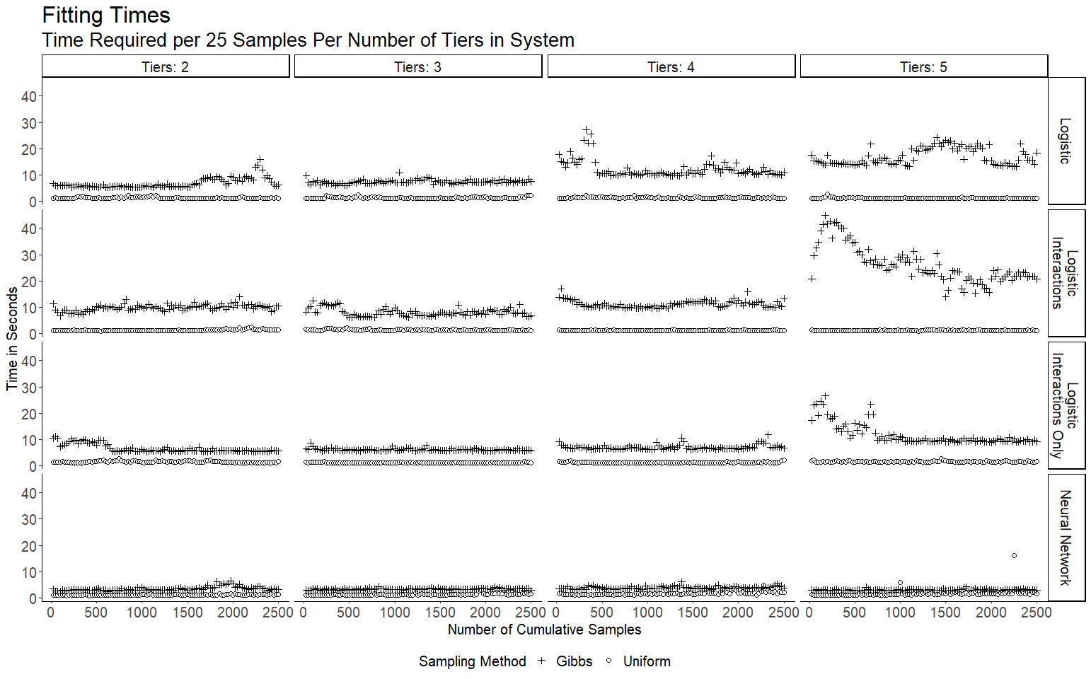
Computational Efficiency
The computational efficiency outcomes are summarized in figure 3 and table 3. As expected, Gibbs sampling is more resource intensive than producing random samples from a Uniform distribution. It appears that the more complex kernels used with logistic regression have longer execution times than linear kernel logistic regression or neural networks, and their execution times scale more rapidly as dimensionality increases.
The instances of neural networks used in this project show the best execution times of all candidate models, and has a much smaller multiple of execution times of Gibbs sampling vs. Uniform sampling than the logistic regression models. This may be due to enhanced implementation procedures, or due to the hyperparameters utilized for these particular models.
Conclusions
In this project we successfully developed machine learning models that can be used to measure systemic risk for system of 87 banks subject to a simplified capital allocation system that allows up to 5 different levels of capital allocation.
| Sampling Method | Gibbs Sampling | Uniform Sampling | ||||||
|---|---|---|---|---|---|---|---|---|
| Tiers | 2 | 3 | 4 | 5 | 2 | 3 | 4 | 5 |
| Logistic Regression | 11.24 | 12.20 | 20.34 | 28.12 | 2.00 | 2.06 | 2.09 | 1.80 |
| Logistic /w Interactions | 16.28 | 13.39 | 18.50 | 43.74 | 1.97 | 2.10 | 1.78 | 1.78 |
| Logistic /w Interactions Only | 10.86 | 10.03 | 11.55 | 19.70 | 2.34 | 1.77 | 1.92 | 2.45 |
| NeuralNetwork | 5.67 | 5.44 | 6.32 | 4.99 | 1.81 | 2.10 | 2.79 | 2.69 |
Table 3: Total Execution Time in Minutes
Our approach builds on the standard Eisenberg-Noe framework, and proves robust enough to to be utilized with logistic regression models utilizing multiple kernels, as well as with basic neural networks.
The research identifies neural networks as the most accurate and efficient models of those considered. It furthers shows that logistic regression with various kernels suffers from poor fits, longer execution times, and presents potential issues regarding monotonicity.
Regardless of modeling approach, Gibbs sampling improves convergence, but at the cost of accuracy using the training data. Overall, the execution times achieved, while long, are favorable compared to simple grid search algorithms.
The models utilized in this project are all parametric in nature and dependent on multiple hyperparameters. The exploration of non-parametric approaches, such as Gaussian regression may provide a more consistent framework for higher dimensions.
Given the relative success of neural networks in the results so far, they could be explored in more detail in future work. Specific areas to consider would be algorithms that better deal with exploding gradients through enhanced backpropagation or gradient clipping methods, and methods that improve monotonicity.
Based on the long execution times of the models, it would be beneficial to consider areas for improvement in code efficiency.
References
Eisenberg, L. and T. H. Noe (2001). Systemic risk in financial systems. Management Science 47 (2), 236–249.