Researchers:
Zichao Li
Tianyi Yang
Faculty Advisor:
Dr. Dan Pirjol
Abstract:
The SABR model is an effective stochastic volatility model for modeling the volatility but option pricing in practical application by finite difference method is time consuming. To solve this problem, artificial neural networks are applied to calibrate SABR parameters by Universal Approximation Theorem for implied volatility. Ann results confirm that ANN works quickly and accurately under the predetermined condition.
Methodology:
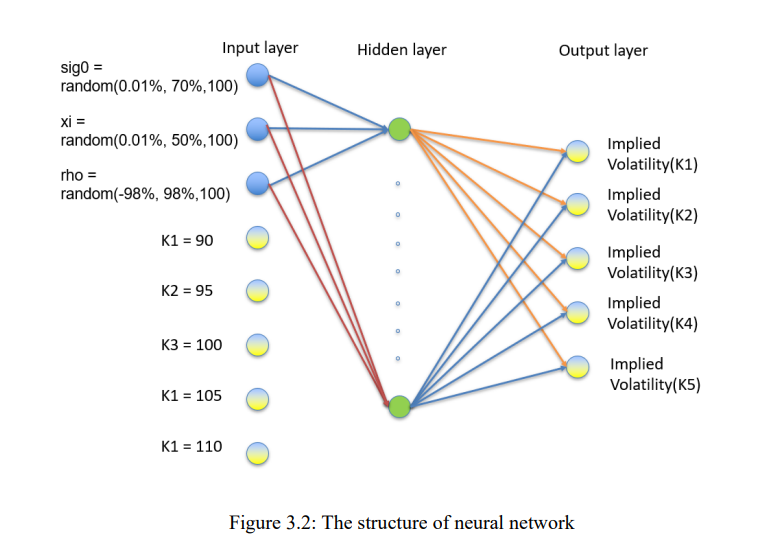
1. Construct the Artificial Neural Network:
The neural network tested in this paper is constructed by only one hidden layer. In the beginning, we set the nodes equal to 1000 and the optimizer function is ‘Adam’, with a loss function of “mean squared error”. The activation function used on the input nodes and the hidden layer is the “softplus” function. Then we use different parametric equations to compare to make our results more accurate
2. Generate Input and Output data:
We set 3 input parameters (𝜎(0), 𝜌, 𝜉) and 5 output implied volatility. For 𝜎(0), 100 numbers are randomly selected from 0.01% to 70%. For 𝜉, 100 numbers are randomly selected from 0.01% to 50%. For 𝜌, 100 numbers are randomly selected from -98% to 98%. Each of the five implied volatility rates corresponds to a strike price [90,95,100,105,110].
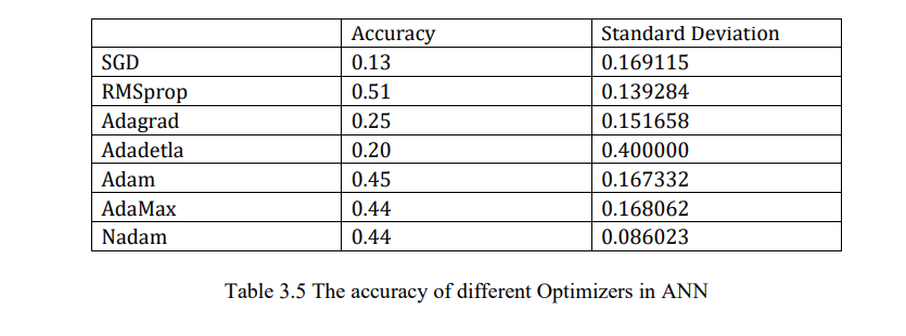
3. Optimizer Algorithm:
The optimizer is used for gradient descent in keras. Gradient descent is one of the most used methods to solve the model parameters of machine learning algorithm. There are many optimizers in keras, such as SGD, Adam and RMSprop,etc. If the input data is sparse, the adaptive learning rate optimization method is recommended. In the adaptive learning algorithm, adadelta, rmsprop and Adam have similar performance results, and Adam is slightly better than the other two algorithms.
Below image shows the accuracy of different optimizers. We can see RMSprop function has the highest accuracy of 51%.
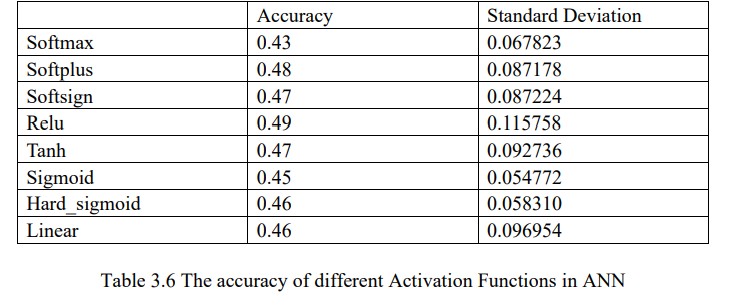
Finally, we used the batch_ Size, epoch and optimizer to choose activation function in Keras. Relu is the best with an accuracy of 49%
Results:
1. Prediction Model Output:
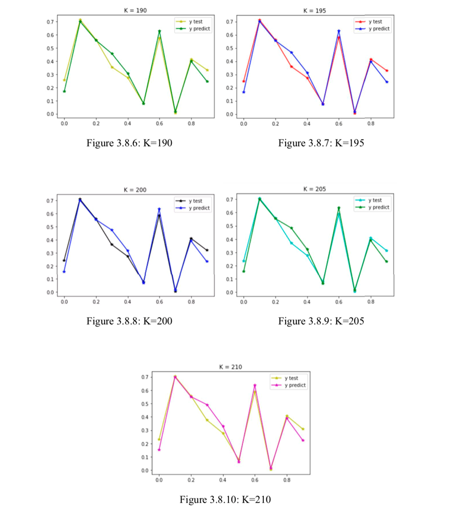
After we have trained our model, we used it to predict implied volatility. We make strike prices same as we used when we calculate training set (K= [90, 95, 100, 105, 110]). Because the strike price is not the input, so we do not need to change it. We use 10 different number for each input parameters, then we got these figures.
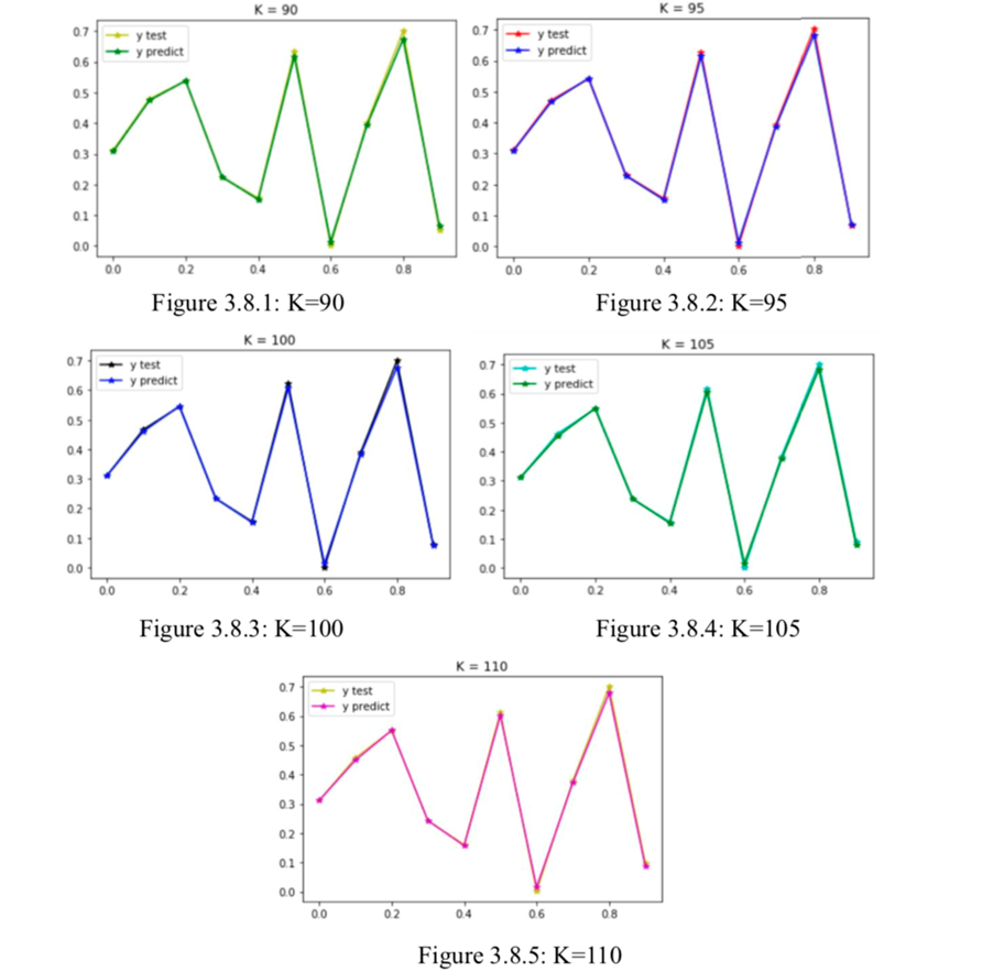
As we can see, the value we predict is almost the same as the real data.
Then we changed our strike price and our stock price, we wanted to make sure our ANN built a SABR model that can be used in different stock prices and strike prices. Then we assume that K= [190, 195, 200, 205, 210] and F=200. The general trend of the predicted value is the same as the true value.
Conclusion
The trained neural network successfully calibrates SABR model parameters and predicts the implied volatility under the predetermined conditions. The SABR approximation is crucial in constructing a training set for the artificial neural network by providing a relational expression between the implied volatility and the SABR parameters (σ0, ξ, ρ). The Universal Approximation Theorem is attributed to the success of the prediction by the feed-forward neural network, which takes input SABR parameters and predicts outputs through weighted sums and activation functions. However, the accuracy of prediction decreases by 80% with an increase in the principal price and strike price and a larger amount of data. Increasing the number of hidden layers may improve the prediction accuracy, and future research can explore multiple volatility surfaces and maturities to test the efficiency and accuracy of artificial neural networks.