
Researchers
Ashley Delpeche, M.S. in Financial Engineering, Graduated in May 2020
Shalini Menon, M.S. in Financial Engineering, Graduated May 2020
Zhentao Du, M.S. in Financial Engineering, Graduated May 2020
Advisor:
Dr. Khaldoun Kashanah
Abstract
For many decades, the relationship between macroeconomic variables and stock prices has been a topic of vast research and experimental methodologies. Hence, the belief that macroeconomic variables have the capability of influencing investment decisions and stimulating further research within its proprietary domain. In this paper, we discuss various economic indicators coupled with their theoretical predictability, in addition to analyzing causality and dependence to the Standard & Poor 500 (S&P500) index, by means of statistical analytical approaches such as Vector Autoregression (VAR), Johansen Cointegration(JC) coupled with Machine Learning methodologies Long Short-Term Memory (LSTM) network and Reinforcement Learning(Q-Learning). Overall, predicted results of the Vector Autoregression model moderately displays a similar relationship to the preliminary data, but implied that very few impulse responses or interdependencies are present amongst the variables. Johansen Cointegration and Q-learning showed strong positive correlations between the actuals and derived estimates, indicating high predictability capacity from both methods for long term forecasting purposes.
Experimental Design & Descriptive Analytics
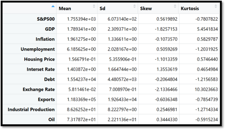
To begin our experiment, data components were obtained from Bloomberg Terminal, encompassing 11 variables, with date range stemming from January 1, 2006 to December 31, 2019. Final selected variables are as followed: Gross Domestic Product (GDP), Inflation, Unemployment, Housing, Interest Rates, Exchange Rates, Exports, Industrial Production, Oil Prices, and Standard & Poor 500 (S&P500).
To further elaborate, final variables were selected based on the below four criteria:
1. The variable would cover half a century or longer, thus showing its relation to business cycles under a variety of conditions.
2. The variable would lead the month around which cyclical revival centers by an invariable interval. 3. The variable would show no erratic movements; that is, it would sweep smoothly up from each cyclical trough to the next cyclical peak and then sweep smoothly down to the next trough, so that every change in its direction would herald the coming of a revival or recession in general business.
4. The variable’s cyclical movements would be pronounced enough to be readily recognized, and give some indication of the relative amplitude of the coming change
Upon retrieving variable data components, we normalized the data using the Jump Method and applied a statistical parameter to obtain significant descriptive analytics. Preliminary descriptive analysis is detailed below in figure 1:
Experimental Results
Method I: Vector Autoregression Using Akaike Information Criterion (AIC)
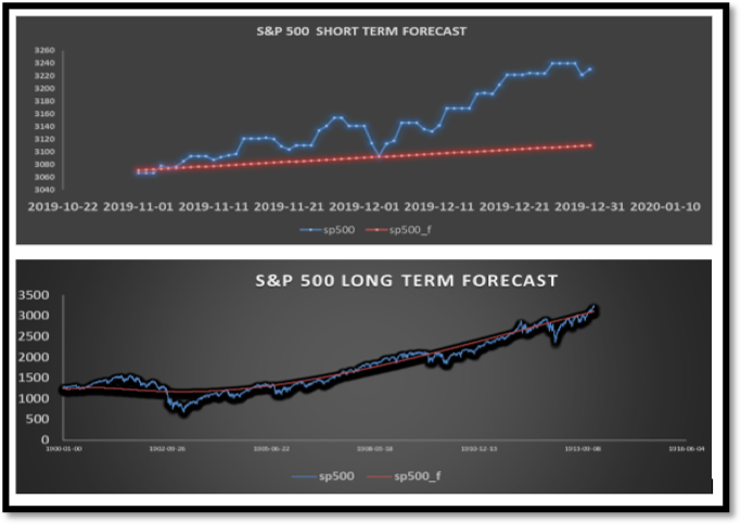
Per the Vector Autoregression methodology, we applied an impulse response to our stationary and first differenced preliminary data, the output displayed that only six variables or pairs would be impacted by a shock from S&P500 – Oil Rate being one of the pairs. Then, we used Akaike Information Criterion (AIC) as our statistical criteria at maximum 32 lags in order to obtain an optimal lag order and AIC results proposes lag 1 as the optimal lag along with the amalgamation of coefficients and system of equations. As a result, Vector Autoregression estimates and forecast values were obtained, and relationships were analyzed accordingly. Per figure 2 below, it is evident that our forecast model is not entirely precise for short term analysis, as it does not capture small fluctuations, but seems to be better suited for long-term predictability analysis.
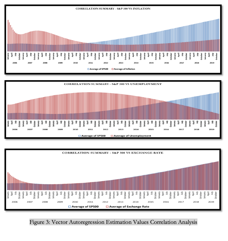
For further substantiation we investigated individual variable relationships, which can be seen in figure 3, and noticed that S&P 500 has a very strong impact on individual variables such as Unemployment, GDP, Housing, and Inflation.
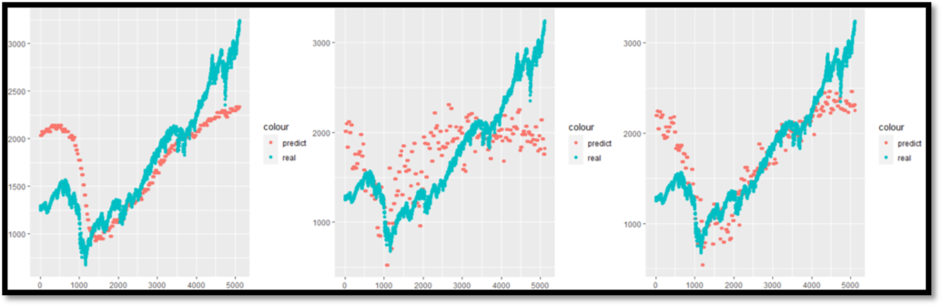
Method II: Johensan Cointegration
For this phase of our experiment, a Trace Test was applied to analyze relationship amongst the variables. Upon application, we discovered that at 1% level the null hypothesis could be rejected between the following
pairs: S&P 500—Housing and S&P 500—Exchange Rate. At the 5% level, we can reject the null hypothesis between: S&P 500—Unemployment and S&P 500—GDP, which means these indicators have a strong impact on the S&P 500. To isolate ‘Leading’ indicators which would enable short- and long-term predictability in this aspect of our experiment, we applied 30 days lagged scenario; the results revealed our leading indicators as GDP, Housing, Inflation and Exchange Rate. Finally, we used different combinations of the leading indicators to forecast the S&P 500 with the results displayed in figure 4. Graph (A) summarizes results that can be rejected at 1% and 5% level and the smoothness of this output may result in small signals being ignored. In graph (B), the results can be rejected at 1% level and is able to catch more small changes, but it does not follow the trend very
well. Thus, we strongly believe the best result is graph (C) because all the result parameters are larger than the critical value and it shows both small changing signals and long trend.
Method III: Long Short-Term Memory (LSTM) network
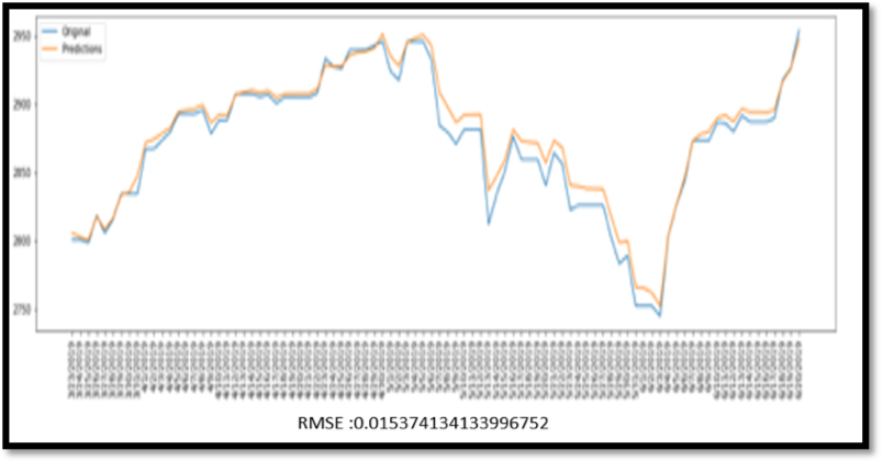
Lastly, the deep learning aspect of our experiment proved that machine learning algorithms can understand the nonlinear relationships between macroeconomic variables and the stock market because it allows them to make highly accurate stock predictions; it is important to note that these models take a multi-dimensional approach. For instance, in this particular scenario, neural network algorithms take all variables into consideration and use them to predict and analyze trends which is displayed in the LSTM model (figure 5), which has a mean square error of 0.01537, where the predicted values very closely mirror the stock market movements.
Method IV: Reinforcement Learning(Q-Learning)
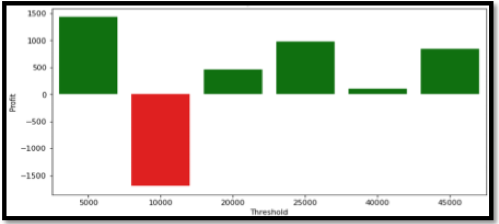
For further validation, we designed a Q-Learning environment to fit our model, which identified its environment as the stock market whose bearing is measured by the S&P 500. We programmed this scenario by cementing the following logic: rewards are the gains with each trade and the punishments are identified as losses. Moreover, we designed a feature to consider the traders risk threshold that would enable trades to take place when losses were within the trader’s threshold and these losses were calculated using Value at Risk (VAR). Our experimental results indicated that the Q-Learning model gets smarter with each trade as shown in the below mentioned histogram (figure 6). To further analyze, Initially, the bot does make negative profits but as the traders are willing to take more risks and more trades take place, the profits are always positive.
Conclusion
As a result of implementing this in-depth and immensely informative experiment, we have noticed that the Machine Learning algorithms provides the most accurate predictions compared to the statistical approaches. Although, Vector Autoregression and Johensan Cointegration can predict the general trends, the neural networks are able to account for the overall trend as well as very small fluctuations. On the other hand, the statistical approaches are able to isolate each variable and measure the significance of its impact on the stock market which can be seen via the Vector Autoregression methodology; also, Johensan Cointegration further validates the results obtained from VAR while diving into which pairs are more significant.