Researchers:
Daniel Beekman
Zongqi Shen
Faculty Advisors:
Dr. Ionut Florescu
Abstract:
Corporate credit rating agencies use quarterly financial statements to estimate a company’s probability of default. These probabilities are categorized into the corporate credit rating system ranging from AAA through D. This paper demonstrates how we can use Credit Default Swap spreads and the KMV model to transform quarterly financial statement data into daily probabilities of default. Using these probabilities of default and classified stock returns to train Logistic Regression and Random Forest Machine Learning models to provide with a daily credit rating. These credit ratings were used to test trading strategies which resulted in a return increase of over 200%.
Methodology:
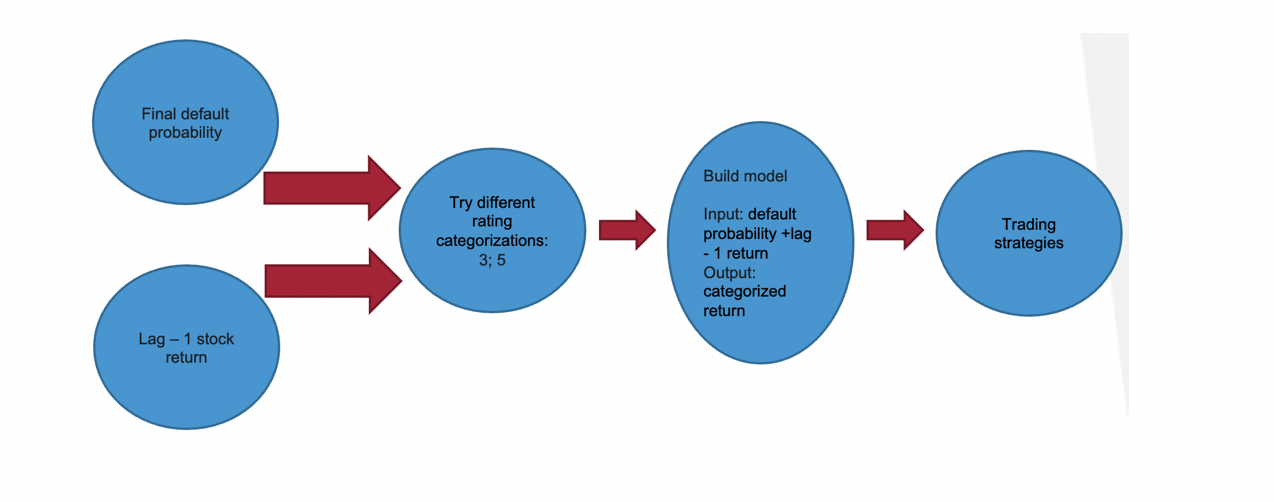
Overview: Aggregate default probabilities implied from Credit Default Swap (CDS) spreads and the KMV model -> Categorize our daily stock returns -> Build a logistic regression model -> Use the predicted values (credit rating) as a decision factor to buy or sell the stock.
- Data Collection: The paper utilizes data spanning from September 30, 2009, to September 30, 2021, and focuses on several companies, including ADM, CL, COST, EL, GIS, KO, MO, PEP, PG, STZ, SYY, and TGT. The data was sourced from Wharton Research Data Services (WRDS) and encompasses information such as Credit Default Swap (CDS) data, daily volatility, and Debt/Asset ratios.
- Default probability from CDS par spread: The default probability from the CDS par spread is determined by finding the coupon rate that sets the CDS's fair value to zero. This coupon rate ensures that the present value of payments matches the expected settlement value in case of a credit event. The probability of default can be calculated using this formula:
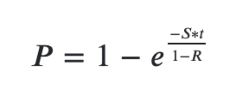
where,
▪ S the spread expressed in percentage terms (not basis points)
▪ t are the years to maturity
▪ R is the recovery rate in percentage terms
3. Default probability from KMV model: This outlines a straightforward method to calculate a firm's credit limit using the KMV model, which considers loan maturity, asset quality, balance sheet structure, and desired default probability. Notable findings include that longer loan maturities result in lower credit limits, higher confidence levels lead to lower limits, and greater asset return volatility reduces credit limits. The paper also provides credit limit estimates for unsecured loans to firms, highlighting its ability to accommodate new debt investments in varying asset qualities. Default probability is determined using the Normal Cumulative Distribution Function of negative distance to default (DD).
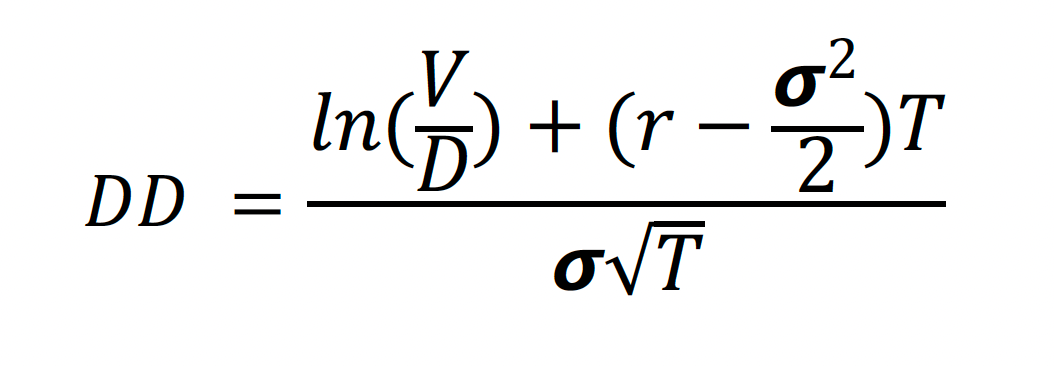
where:
V = value of a firm, D= debt of a firm, r = risk free rate, 𝞼 = annual volatility of stock return, T = time
4. Default Probability Aggregation: Testing of three different methods of aggregation to create our X1: higher, mean, or lower of the two default probabilities.
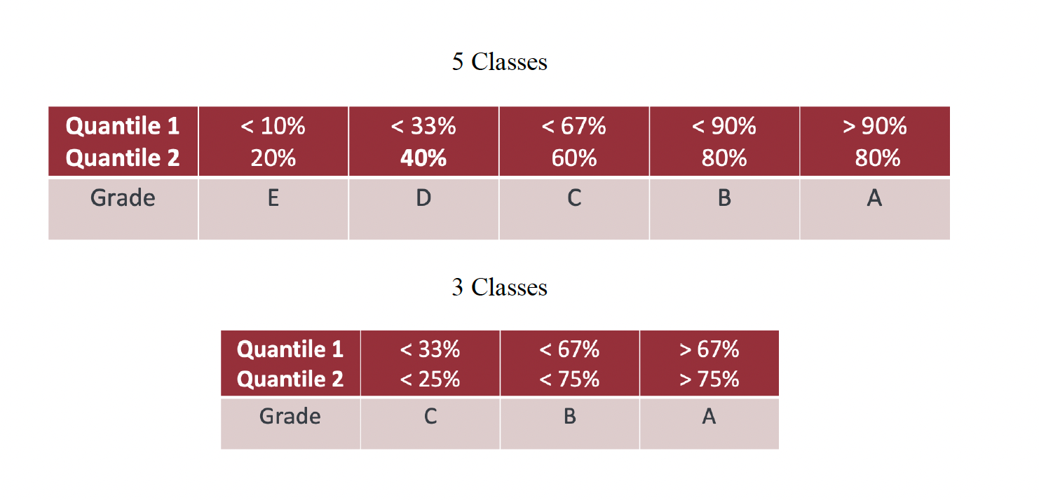
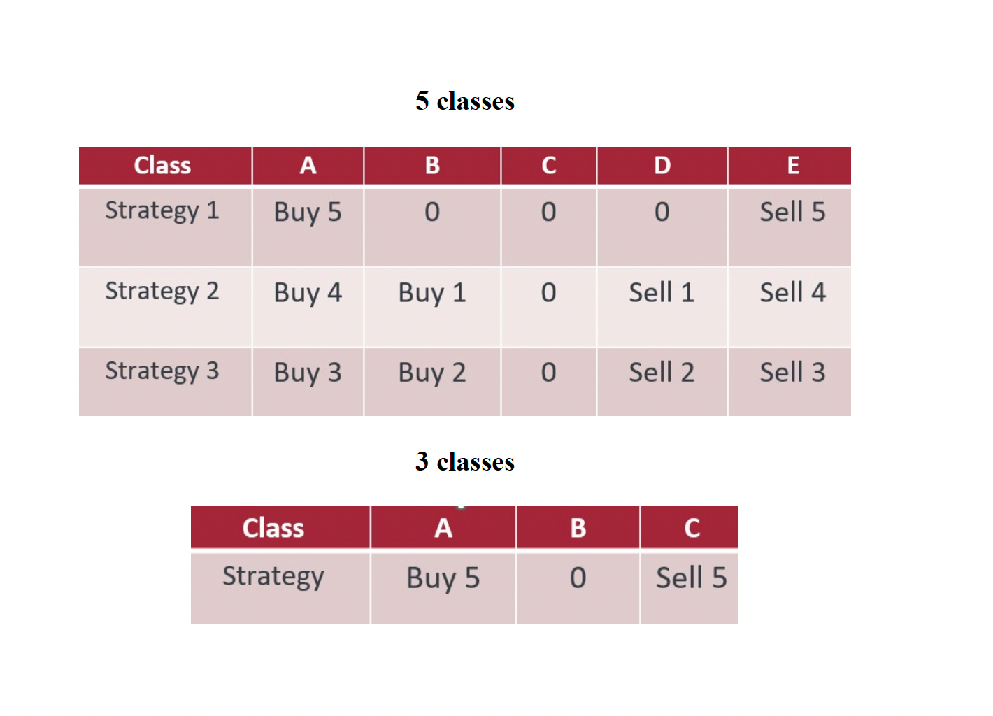
5. Transforming Stock Returns into a qualitative variable: To shift from a quantitative to qualitative variable, begin by choosing the number of classes. Next, determine the relevant quantile for each class. Conduct distinct tests with both 5 and 3 classes, and employ two different quantile divisions for each. Categorize the stock return according to the tables provided below.
6. Logistic regression is a statistical technique for predicting binary outcomes, like yes or no, based on past data. It models the relationship between one or more independent variables and a dependent variable. Logistic regression is a widely used classification algorithm, particularly effective when dealing with linearly separable classes. It relies on the Sigmoid or Logistic function to make decisions, as it produces probabilities between 0 and 1.
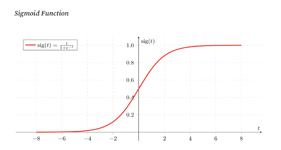
For binary classification tasks, the Sigmoid function is applied in the output layer. In multi-class scenarios, an extension of the One-vs-All approach is used, encoding target class labels through one-hot encoding. For class label prediction, the "argmax" (index with the highest value) is returned. If meaningful class probabilities, which sum to 1, are needed, the SoftMax function, also known as "multinomial logistic regression," is employed. SoftMax computes the probability of a sample belonging to a particular class by normalizing the sum of all linear functions.
7. Trading Strategy and Measure of Success: The credit ratings (representing predicted stock return classes) are the pivotal determinants in the trading strategies. Three strategies are employed for the five-class rating, while a single strategy is used for the three-class rating. The choice of an odd number of classes was made because all strategies mandate inaction when the credit rating aligns with the median class (C for five classes, B for three classes). The subsequent table outlines the actions prescribed at each time point.
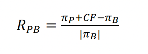
The trading environment is initiated with an initial holding of 100 shares for each stock. At every time increment and for each company, actions are executed according to the decision table's instructions. The resulting monetary gains or losses from these transactions are recorded. Upon completion of all actions, the final portfolio value is assessed and compared to the benchmark value. The benchmark represents the portfolio's worth containing 100 stocks without any trading actions. The relative portfolio return compared to the benchmark is expressed as:
Conclusion:
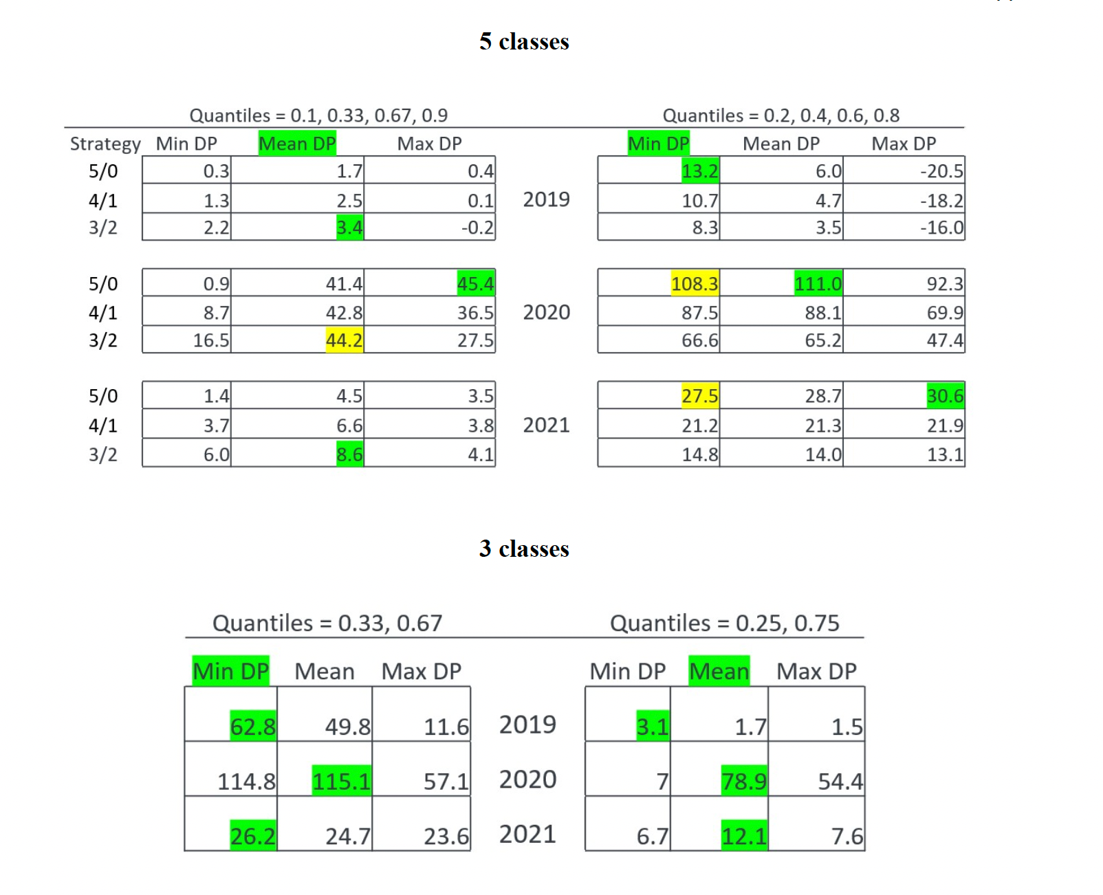
This study examined 12 models using 4 classification methods and 3 aggregation techniques over three years: 2019, 2020, and 2021. A graph highlighted prediction accuracy for model development and testing. The analysis focused on three aggregation methods (Mean, Maximum, Minimum) for default probability and four stock return classification methods, totaling 12 test models. Notably, two scenarios were explored: one with five rating categories in 2021 testing and another with 2019 testing. In 2021, the low default probability aggregation method led to high accuracy for CL company, but in 2019, it resulted in the lowest accuracy. In 2019, only 4 out of 24 model-strategy combinations had lower returns than the benchmark, all from the 5-class categorization. These were related to the 3/2 strategy with max default probability in quantile 1 and three others from max default probability in quantile 2. The least successful predictions occurred when classes were evenly distributed, except when class C was the sole prediction. The best method was the 3-class categorization with minimum default probability, achieving a total return of 204% over three years.